Getting started
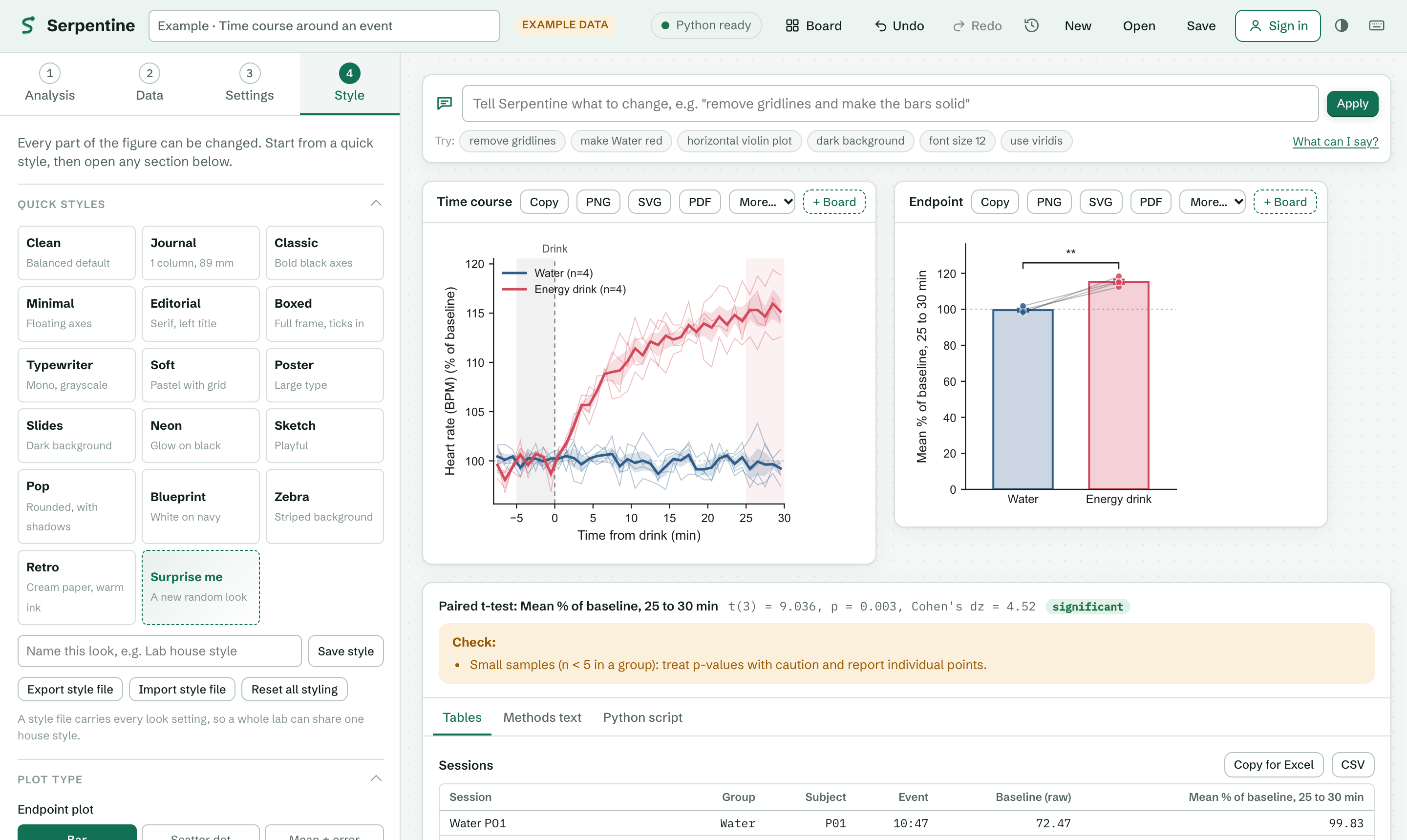
Open Serpentine and wait for the status at the top right to read Python ready. The app opens with an example loaded so you can see a finished analysis right away.
The left column has four numbered steps: Analysis, Data, Settings and Style. Work through them in order the first time; after that, jump to any step. The right side shows your figures, results and tables, and updates as you go.
Not sure which analysis you need? Type into the search box above the list (for example ELISA, half-life or qPCR), or press Help me choose and answer two or three plain questions.
Press Example on any analysis to load sample data for it. It's the quickest way to learn what each setting does.
Choosing an analysis
| If your question is… | Use |
|---|
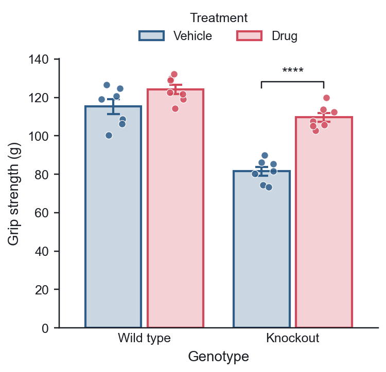
| Do these groups differ? | Compare groups. Control vs treatment, several doses, genotypes, before vs after in the same subjects. |
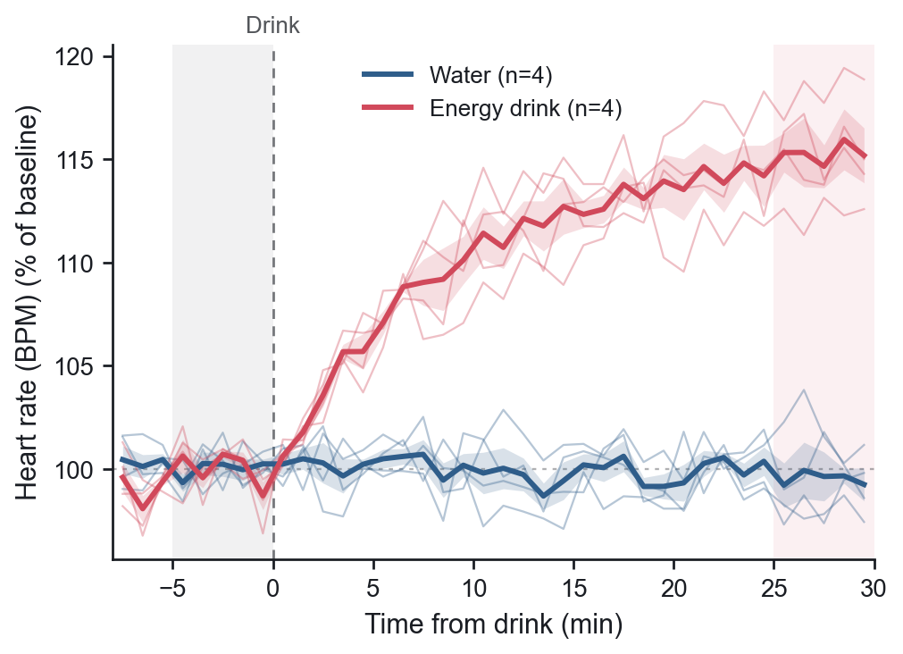
| How did a signal change after an event? | Time course around an event. Breathing, heart rate, blood pressure, temperature, activity or any recording with a time column. |
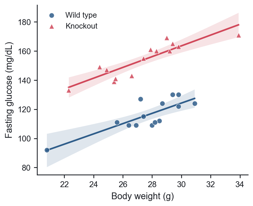
| Does one measure track another? | Correlation & regression. |
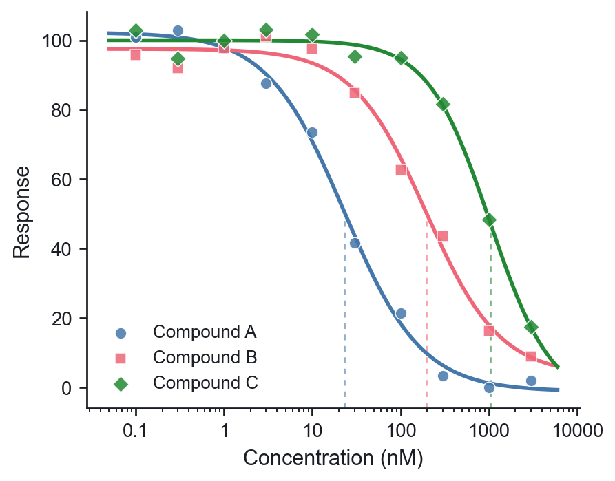
| How potent is this compound? | Dose-response curve. |
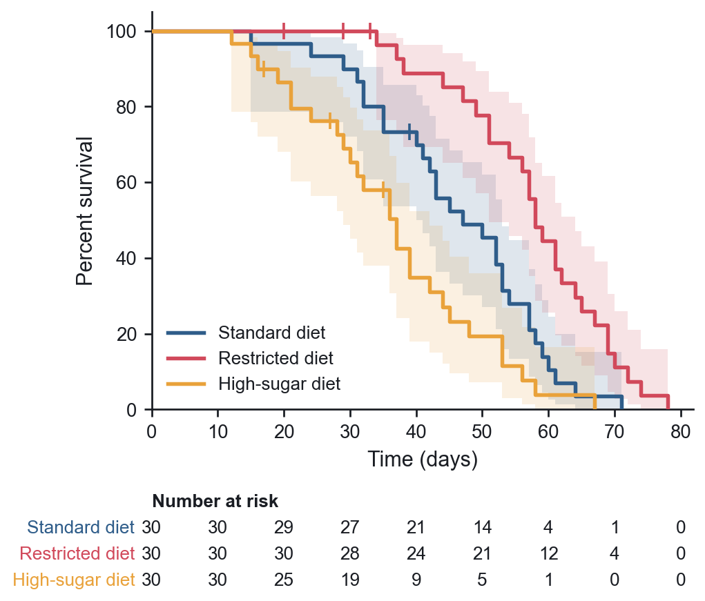
| How long until death, relapse or another event? | Survival curve. One row per subject with its time, whether the event happened (1) or it was censored (0), and its group. |
| Do two factors, like genotype and treatment, interact? | Two-way ANOVA. One row per value with both factors, or a Prism-style grouped table. |
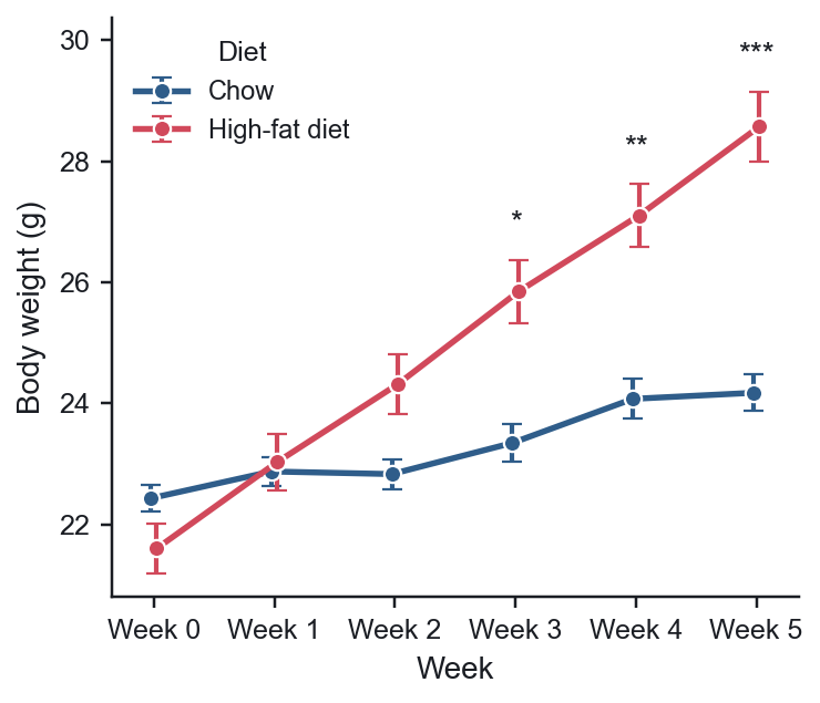
| How did the same animals change over weeks, by group? | Repeated measures. One row per measurement with subject ID, group, time point and value. |
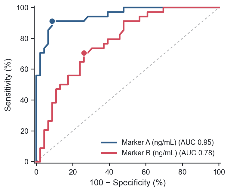
| How well does a marker detect disease? | ROC curve. One row per subject with the true outcome and the marker values. |
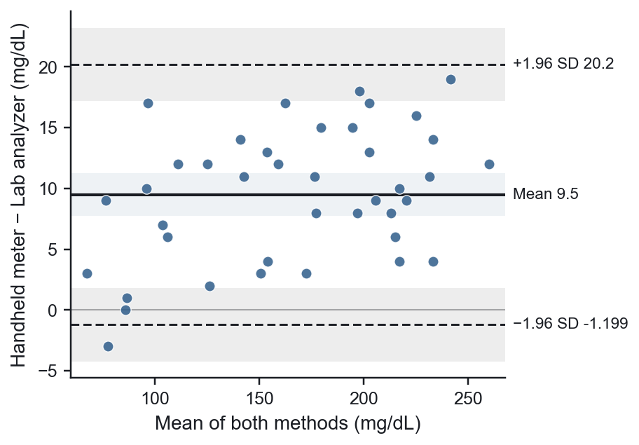
| Does a new method agree with the old one? | Method comparison. One row per sample measured by both methods. |
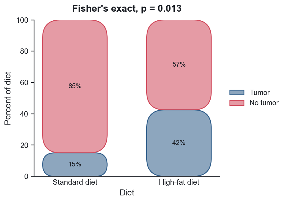
| Did more animals respond in one group? | Counts & proportions. A table of counts, or one row per subject. |
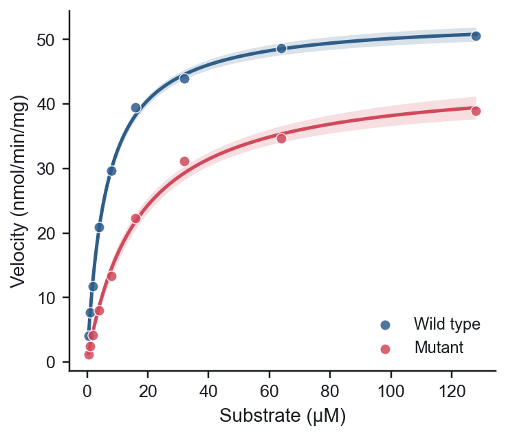
| What is the Km, half-life or doubling time? | Curve fitting. Pick a model or type your own equation. |
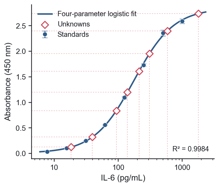
| What concentration is in my samples? | Standard curve. Standards with known concentrations, unknowns with the concentration left empty. |
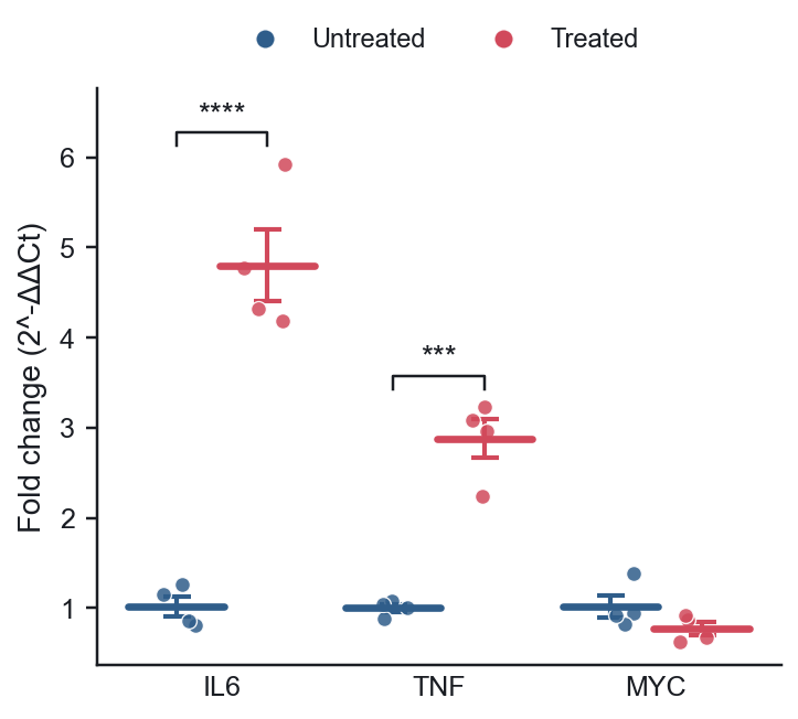
| Did gene expression change? | qPCR gene expression. The Ct export from your instrument. |
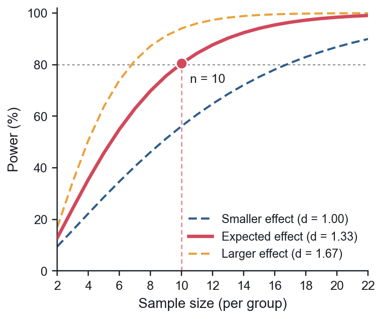
| How many subjects do I need? | Sample size & power. No data needed. |
| Not sure? | Press Help me choose above the analysis list. |
Adding data
In the Data step, either press Paste a new table and paste into the box, press ⌘V / Ctrl+V anywhere on the page, or drop files onto the dashed area. CSV, TSV, TXT and Excel files work. Each Excel sheet becomes its own table.
Put column names in the first row. Serpentine shows how it read your table underneath, labelling each column as number, time or text, so you can check it before going on.
Compare groups: two layouts
One column per group (like Prism's column tables):
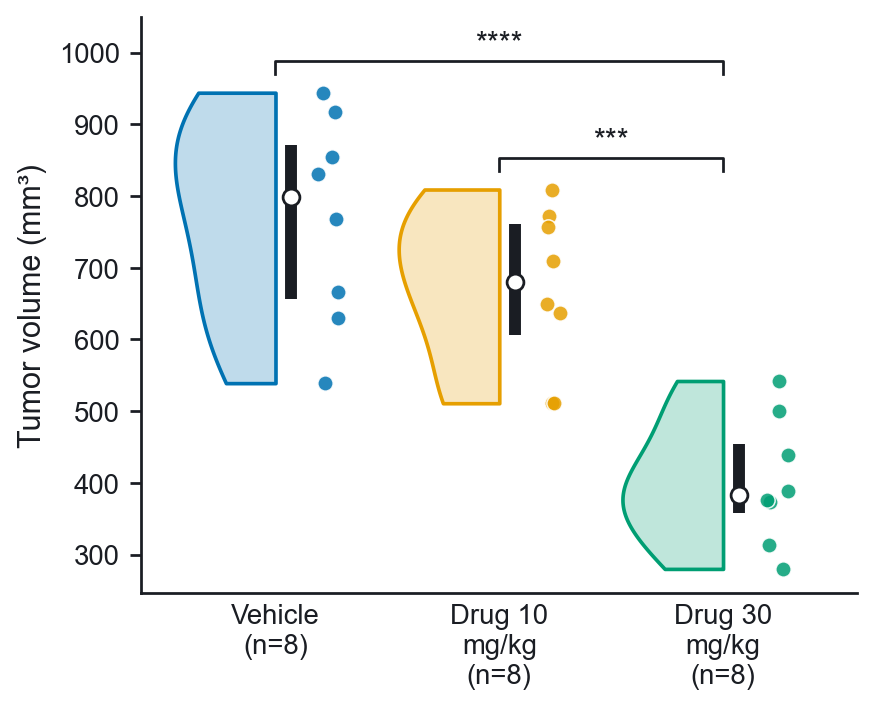
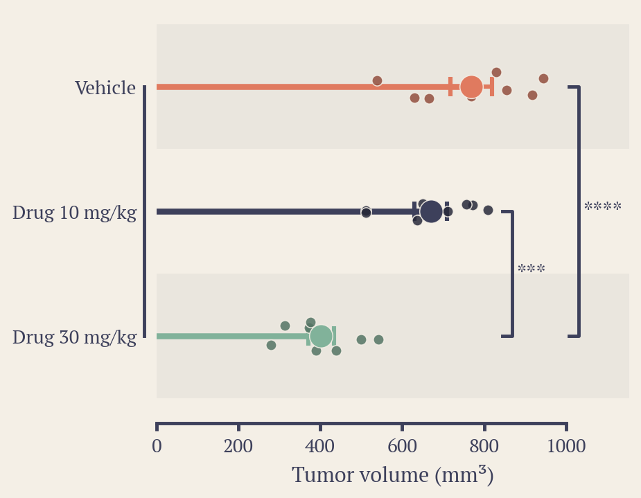
Vehicle   Drug 10 mg/kg   Drug 30 mg/kg
812       640             395
905       702             410
…
Values plus a group column (tidy format, common in exported data):
Mouse   Genotype   Weight (g)
M1      WT         26.1
M2      KO         29.4
…
From LabChart
In LabChart, select the rows of your Data Pad, copy them, and paste into Serpentine. Channel, measurement and unit rows become tidy names like Cyclic Rate (BPM), and time columns written as 8:40 or 0:08:40 are read as clock times automatically. If you marked the injection with a LabChart comment, Serpentine uses that comment's time as the event, so you don't have to type it.
From Prism
Grouped tables with several replicate columns under one heading (Control: Rep 1, Rep 2, Rep 3) are combined into one group per heading. Turn this off in Settings if you want every column on its own.
From a plate reader
Press Import a plate in the Data step. Paste the block of readings from any plate reader's export (96 or 384 wells, with or without the A–H letters and 1–12 header), and optionally a plate map in the same layout saying what is in each well:
     1          2          3          4
A    Std 1000   Std 1000   Control 1  Control 1
B    Std 500    Std 500    Control 2  Control 2
…
H    Blank      Blank
Standards are labelled Std 250 or just the concentration, blanks Blank or B, and wells with the same label are replicates. Empty wells are skipped. A live plate preview shows how each well was read. With standards, the table goes straight into a Standard curve with the blank subtracted; without them, choose one row per well or one column per sample for Compare groups.
Technical replicates
If each animal, culture or well was measured several times, use the values + group layout with a column naming the subject, and set Replicates nested in to that column in Settings. Replicates are averaged per subject first, so the test counts biological replicates instead of inflating n (pseudoreplication).
Time-course sessions
For a time course, add one table per recording session. Every session needs the same column names. A sessions sheet then appears in the Data step, where you fill in four things for each one:
| Field | What to enter | Example |
|---|
| Group | The condition this session belongs to. | Treated |
| Subject | The animal or participant. Used to pair sessions from the same subject. | M101 |
| Event | When the injection or stimulus happened, in recording time. Use mm:ss, h:mm:ss or seconds. | 10:30 |
| Exclude | Time ranges to drop, such as a loose wire or movement. Separate several ranges with commas. | 8:00-8:50, 21:10-22:00 |
In Settings, choose the measurement, the bin size, the baseline window (for example −5 to 0 min), how to express values (% of baseline, change from baseline, fold, or raw) and the endpoint window that gets tested. A quality column filter lets you keep only rows that pass a check, for example a cycle count of at least 10.
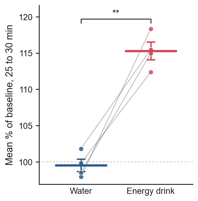
Turn on Pair sessions by subject when the same animals were recorded under each condition, so Serpentine uses a paired test.
Filling in the sessions table quickly
- Fill group & subject from names: name your tables like
Treated 07 or Control_P01 and one click fills in the group and subject.
- Paste session details: paste a small sheet from Excel with columns such as
Session, Group, Subject, Event and Exclude. Rows are matched by session name (or in order if there's no Session column).
- Sessions still missing an event time are highlighted. Times found in a comment column appear in grey, and anything you type overrides them.
If a window doesn't fit your recordings, Serpentine says so and suggests one that does, for example “Recordings end about 10 min after the event; try an endpoint from 5 to 10 min.”
How tests are chosen
With Test: Automatic, Serpentine checks each group with the Shapiro-Wilk test. If every group looks normal it uses a parametric test, otherwise a rank-based one. You can force either choice.
| Design | Parametric | Non-parametric |
|---|
| 2 groups | Welch's t-test (or Student's) | Mann-Whitney U |
| 2 paired | Paired t-test | Wilcoxon signed-rank |
| 3+ groups | One-way ANOVA + Tukey or Dunnett | Kruskal-Wallis + Holm-corrected Mann-Whitney |
| 3+ paired | Repeated-measures ANOVA + Holm-corrected paired t | Friedman + Holm-corrected Wilcoxon |
Effect sizes (Hedges' g or Cohen's dz) are reported for two-group tests. Groups with fewer than five values trigger a reminder to show individual points and interpret p-values carefully.
Repeated measures over time
When the same subjects are measured at several time points, use Repeated measures (or add a subject column in Two-way ANOVA). Serpentine works out the design from the subject IDs: a mixed design when each subject stays in one group, or repeated measures on both factors when every subject gets every combination. Sphericity is corrected with Greenhouse-Geisser by default (ε is reported), comparisons within the same subjects use paired t-tests, and Šidák or Holm corrects for multiple comparisons. Results match pingouin and SPSS.
Styling figures
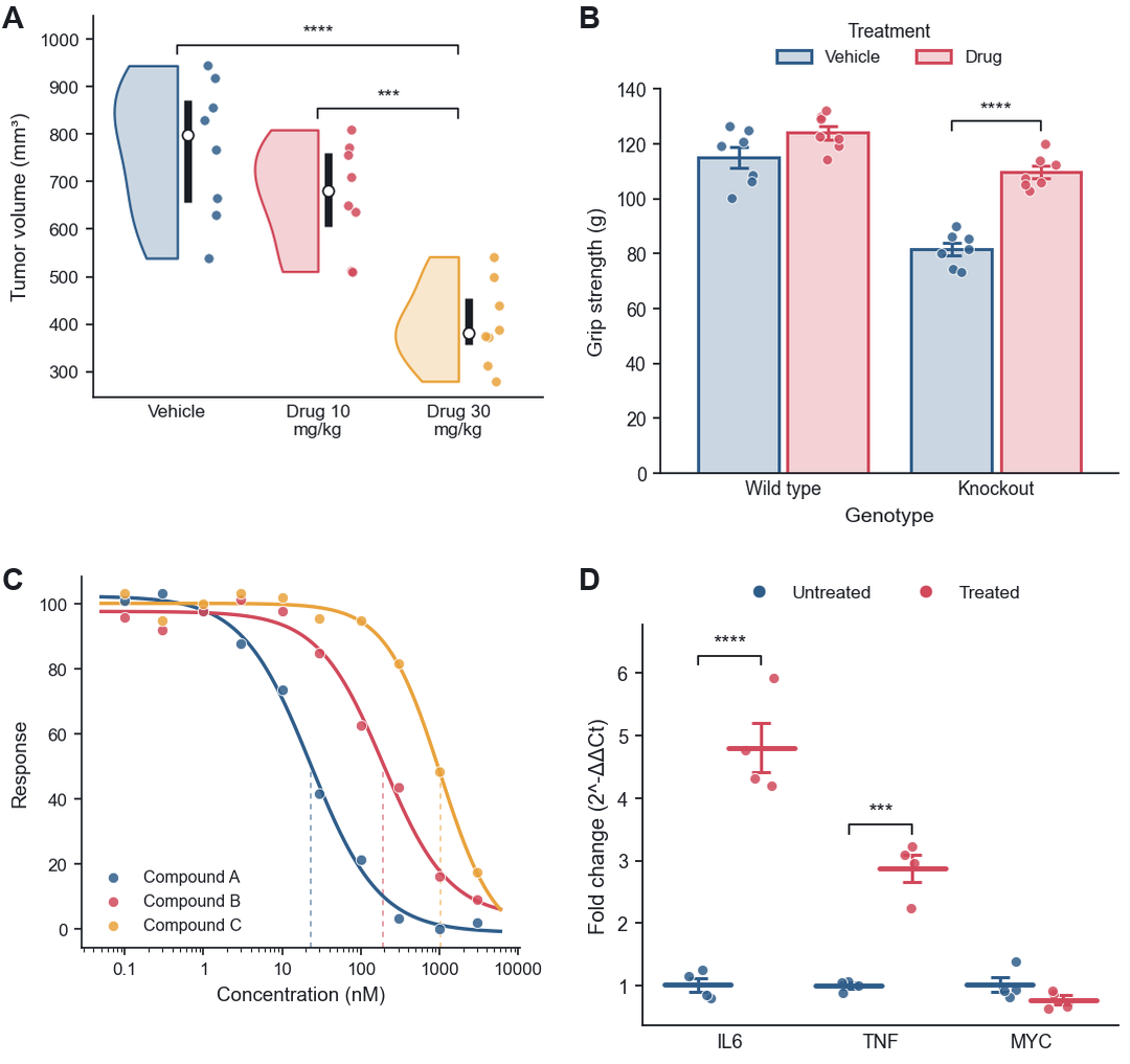
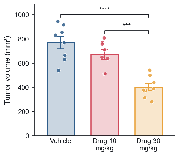
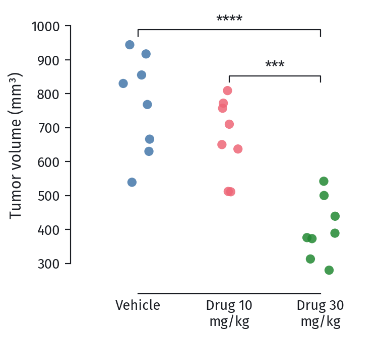
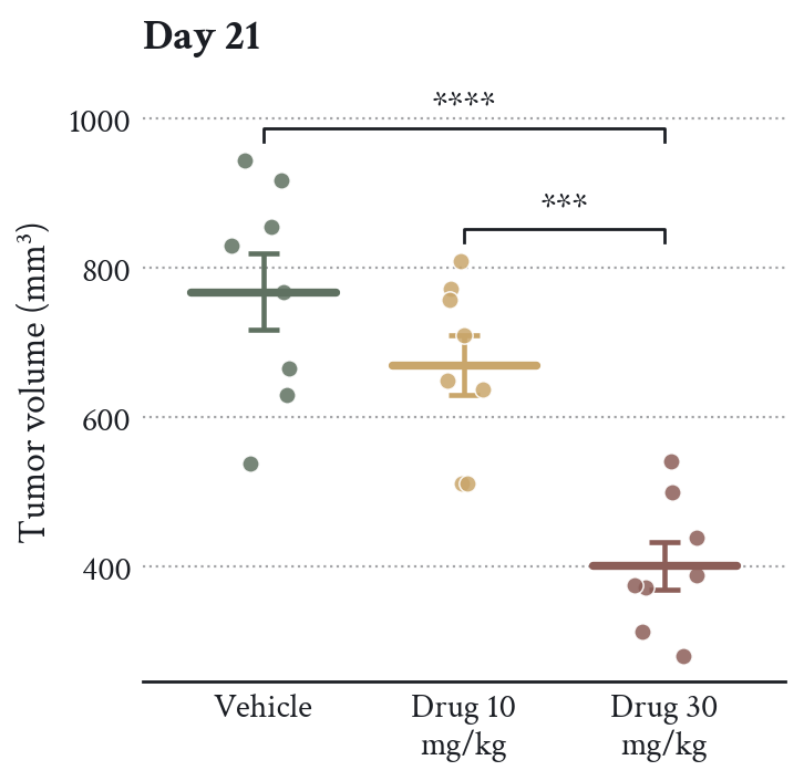
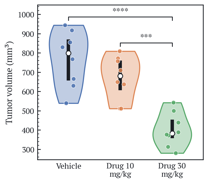
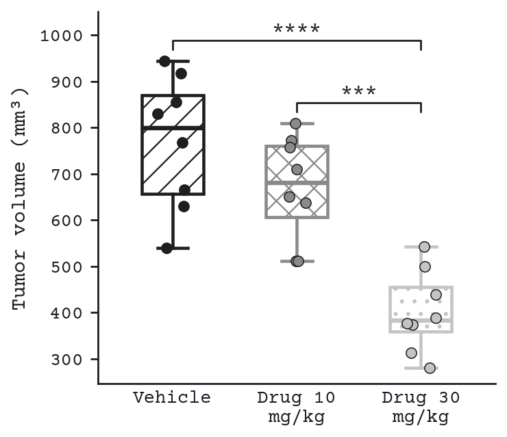
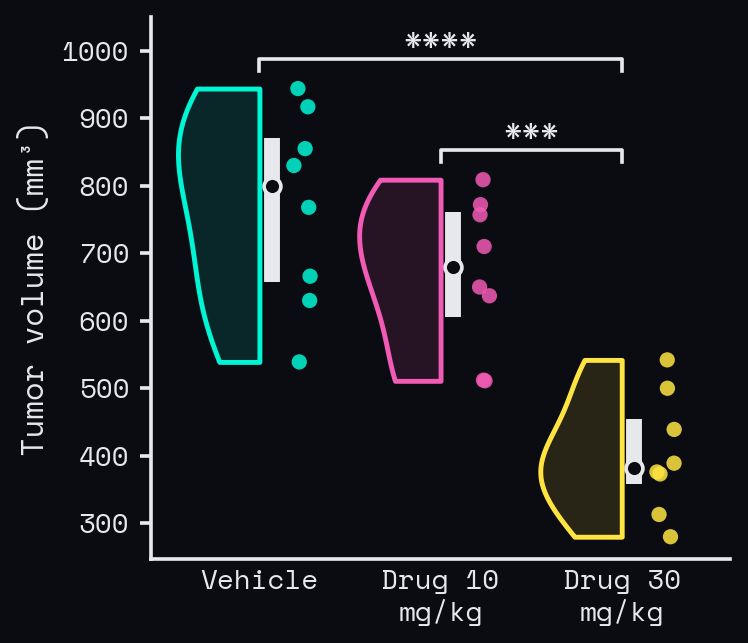
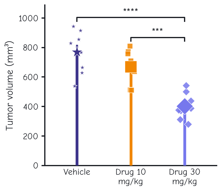
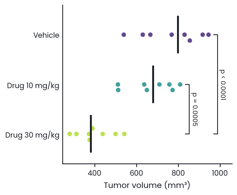
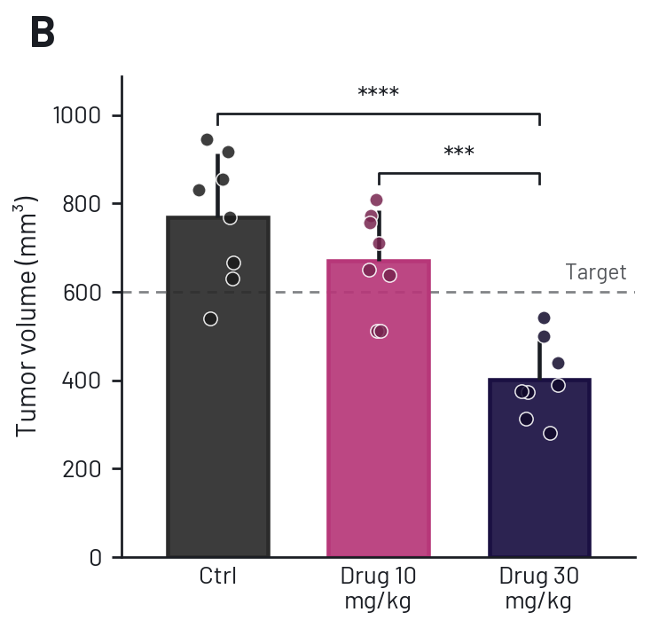
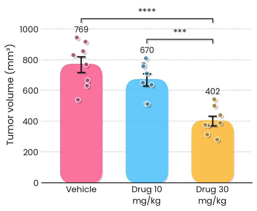
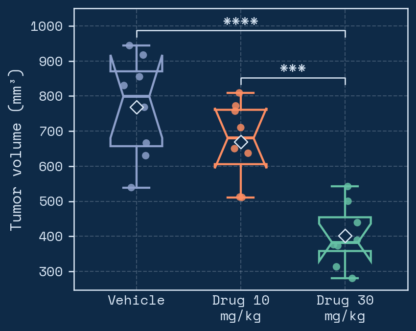
The Style step has everything you would otherwise do in matplotlib, in collapsible sections. Start with a quick style (Clean, Journal, Classic, Minimal, Editorial, Boxed, Typewriter, Soft, Poster, Slides, Neon, Sketch, Pop, Blueprint, Zebra or Retro), or press Surprise me for a random look, then change anything:
- Plot type: bar, scatter dot, mean ± error, box, violin, box + violin, raincloud, beeswarm, strip or lollipop, vertical or horizontal, with adjustable widths, point spread, fill and outline, rounded bar corners, notched boxes, a mean marker and numbers (mean, median or n) above each group.
- Effects: flat, drop shadows or a glow, and an optional striped background.
- Groups: rename any group and give it its own color, marker, hatch pattern and line style.
- Colors: palettes, any matplotlib colormap (reversible), your own hex codes, and separate figure, plot-area and text colors.
- Points, lines and error bars: marker shape, size, opacity and outline; line and axis widths; SEM, SD or 95% CI, two-sided or outward, with any cap width.
- Text: twelve fonts, separate sizes for title, axis labels and ticks, bold options, title position, label angle and a panel letter.
- Axes: choose each axis line, offset and trim them, tick direction, length and spacing, minor ticks, decimal places, limits and log scales.
- Grid, reference lines and legend: gridline direction and style; lines such as
y=100: Baseline; x=0; legend position, columns, frame and title.
- Size: width and height in inches with millimetres shown. Journal style fits a single 89 mm column.
Plain-English commands
Above your figure is a command bar. Type what you want and press Enter, for example remove gridlines, make Water navy and Energy drink coral, horizontal violin plot, y axis from 0 to 1000 or title Day 21. Combine several with “and” or commas. Serpentine shows exactly what it changed, and What can I say? lists the kinds of commands it understands. It runs on your computer, so it's instant and private. Press ↑ to bring back an earlier command.
Commands know your column names too: use heart rate, quality column signal quality at least 80, plot glucose against weight, color by genotype, only Control and Treated.
Commands also reach the analysis itself and a few actions: baseline from -2 to 0, 10 second bins, use the nadir, percent of control, use a nonparametric test, put Energy drink first, export as pdf. Describe a feel, like make it look professional or for my presentation, and it picks a matching style. Small typos are corrected, and when it can't tell what you meant it suggests the closest commands.
Your own styles
Name the current look and press Save style to reuse it in any project. Export style file saves it as a file that colleagues can import, so a lab can share one house style.
Advanced: Python
The last section accepts matplotlib settings (one key: value per line) and your own Python code, which runs on each figure with fig, ax, plt, np and pd ready. For example ax.set_yticks([0, 50, 100]). Errors appear as notes instead of breaking the figure, and your code is included in the downloaded Python script.
Changed your mind? Undo and Redo (⌘Z / ⇧⌘Z) step back through every setting.
Exporting results
- Figures: PNG, SVG and PDF buttons on each figure, with TIFF, JPG and EPS under More. Copy puts the figure on your clipboard for slides and documents. Set resolution and a transparent background in Style.
- Tables: Copy for Excel puts a table on your clipboard to paste into Excel or Prism; CSV downloads it.
- Methods text: a paragraph describing what was done. Treat it as a draft and check it against your protocol.
- Python script: a single file that reproduces the analysis. Run it with
pip install numpy scipy pandas matplotlib then python script.py.
- Report: the Report button above the results opens one page with the results, notes, every figure, the methods and all tables, ready to print or save as a PDF for a lab notebook or meeting.
- Share link: Share link makes a link that opens a copy of the whole analysis (data, settings, style and board) in anyone's browser. It's encrypted with a key that exists only in the link, so the server can't read it. Choose how long it works (1 day to 1 year) and remove it any time. Making links needs a free account; opening them doesn't.
Multi-panel figures
Press + Board above any figure to add it to the figure board, then open Board in the top bar. Panels can come from different analyses and different data, so a dose-response curve, a time course and a bar chart can sit together in one figure.
- Choose 1 to 4 columns and a journal width: single column (89 mm), 1.5 columns (140 mm), double column (183 mm) or poster.
- Pick the panel letter style (A, a, A), (a)) and size, and the gap between panels.
- Reorder panels with the arrows. Edit loads a panel's data and settings back into the main window; change anything, then press Update panel on the figure.
- Export the whole figure as PNG or TIFF (300 to 1200 dpi), PDF, or SVG for editing in Illustrator or Inkscape. Each panel is redrawn at full quality.
Saving projects & accounts
Serpentine keeps your latest work in this browser automatically. You can also keep it for good in two ways.
As a file. Without an account, Save (⌘S / Ctrl+S) downloads a .serpentine.json file with your data and every setting. Open loads it again on any computer.
In your account. Press Sign in at the top right and create a free account with your email and a password. Then Save stores the project online, and every change after that saves automatically; the dot next to your name shows Saved online. Open your projects from any computer under your name in the top bar. Your saved styles go with you too.
End-to-end encrypted. Projects are encrypted on your computer with your password before they're uploaded, so the server only ever holds scrambled data that nobody else can read, including whoever runs Serpentine. That's also why nobody can reset your password for you: when you create an account you get a recovery key. Download it or write it down. With it, Forgot password? lets you set a new password; without it and your password, your online projects can't be opened.
- Two tabs or computers: if a project changed somewhere else since you opened it, Serpentine asks which version to keep instead of overwriting.
- Account settings: change your password, get a new recovery key or delete your account and everything stored online.
- Signing out removes online projects from that browser, which is useful on shared lab computers.
- Online storage is 200 MB per account. Large time-course projects are compressed before they're encrypted.
Undo & shortcuts
Undo and Redo cover everything: settings, styles, data tables, examples, opening projects and the figure board. Undo tells you what it reverted, and the clock button next to Redo lists recent steps so you can go back several at once.
| Keys (Mac / Windows) | Action |
|---|
| ⌘Z / Ctrl+Z | Undo |
| ⇧⌘Z / Ctrl+Y | Redo |
| ⌘S / Ctrl+S | Save (online when signed in) |
| ⌘O / Ctrl+O | Open a project file |
| ⌘E, ⇧⌘E, ⇧⌘C | Export the first figure as PNG, as SVG, or copy it |
| / or ⌘K | Type a plain-English command |
| 1 – 4 | Go to Analysis, Data, Settings, Style |
| B, + | Open the figure board, add the figure to it |
| H, T, ? | Undo history, switch theme, show all shortcuts |
Single-letter shortcuts work when you're not typing in a field. While typing, ⌘Z undoes your text as usual.
Troubleshooting
- Stuck on “Starting Python”. Serpentine needs an internet connection to load the Python engine the first time. Check your connection and reload.
- A column reads as text. Usually a stray word inside the numbers. Values with units attached, such as
48.2 mL/min, are read as numbers automatically.
- “Time jumps back” note. A new LabChart block restarted the clock at 0:00. Serpentine keeps the first block; paste later blocks as their own session if you need them.
- “Couldn't read the time”. Write event and exclusion times as
10:30, 0:10:30 or plain seconds like 630.
- The downloaded copy shows a blank page. Start it with the launcher file rather than opening
app.html directly, because browsers block the Python engine on pages opened from disk.